The Footprint of a Use: Per Query, Per Task and Per Agent
Chapter 5 counted the footprint of a model. This chapter counts the footprint of a use, which is the quantity an organisation decides about and the unit in which Chapter 4 told you to manage. A use is one defined application of AI that someone owns, such as the citizen-service assistant or the claims-triage agent. Its footprint is the footprint of one unit of work (a query, a task, an agent run, a resolved enquiry) multiplied by the number of units. Both factors can be wrong by a large amount, and the first more often than the second, because published figures for one unit of work rest on boundaries that differ and on multipliers that a headline number hides. The chapter belongs to E1 Measure. It is the Count test of the net-benefit principle applied to one use, and it says nothing yet about whether the use is worth its footprint (E2 Justify, Chapter 9) or about how to reduce it (E3 Design, Chapters 12 to 16).
The core finding is that the same prompt, answered by the same service in the same month, gives numbers a factor of two to three apart depending on where the boundary is drawn, and that a use that reasons at length, reads a long context or runs as an agent can differ from that prompt by one or more orders of magnitude. A provider's per-prompt figure is context. The footprint of your own use is a record you build at a boundary you chose, with a range you state. Figure 6.1 shows where the multipliers enter. The chapter gives the method, the boundaries that must never be compared, and the footprint record (FPR) in which the result is kept.
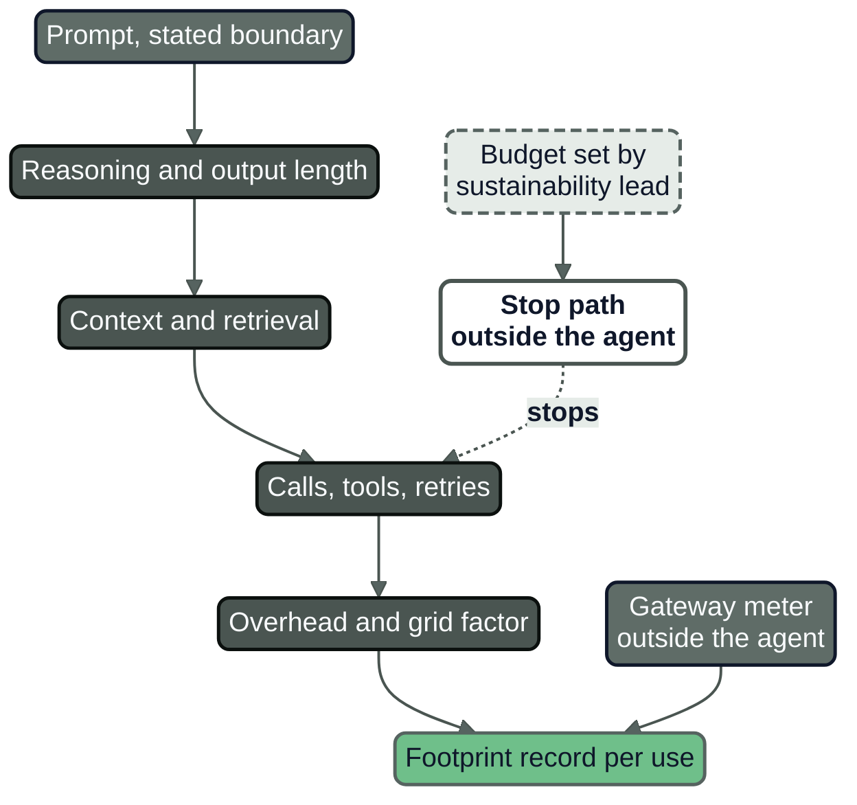
Figure 6.1: From a single prompt to an agent run. The multipliers enter in the order shown; the gateway meter, the budget and the stop path sit outside the agent. No figure is carried by the diagram.
The unit of decision
Decisions are made per use: whether to launch it, which model it runs on, how long its context may grow, how many calls an agent may make, and where it runs. Footprint per use times volume is what the organisation manages (Chapter 4), so the chapter starts with the use and its functional unit.
The functional unit is the unit of work whose footprint is counted, chosen so that it is the same unit that the benefit is measured in. AI Platform and Security, Chapter 22 chose the unit for cost: the Software Carbon Intensity (SCI) specification of the Green Software Foundation, published as ISO/IEC 21031:2024, divides emissions by a functional unit that should be the one used for cost, such as a resolved enquiry or a processed claim (21, Green Software Foundation, 2024), as AI Platform and Security, Chapter 22 does (27, Nordqvist, 2026). This book keeps that choice and extends it. Chapter 5 explains when a per-use unit is a functional unit in the life cycle assessment sense. Four units recur, and each answers a different question:
- A query (or request) is one prompt and one completion. It is the unit of provider disclosures and of benchmarks.
- A task is what a person or a system set out to get done, which may take several queries: a drafted letter, a summary with a follow-up, a resolved enquiry.
- A run is one execution of an agent from the moment it starts work to the moment it stops, with all its model calls, tool calls, retries and background work.
- An outcome is the task completed successfully, with failed attempts counted in the numerator. It is the unit that matters when the benefit is the result and not the activity.
The distance between a query and an outcome is where most of the error sits. A resolved enquiry at Nordvik Region needs more than one query (a question, a retrieval, a generation, sometimes a clarification), and a claim triaged at Hansa Mutual needs an average of nine model calls (the profile in docs/EXAMPLE_ORGANISATIONS.md). A per-query figure multiplied by the number of enquiries therefore understates the footprint by the number of queries per enquiry.
The rule of this chapter is that a use's footprint is recorded as the footprint of its functional unit with a stated statistic (median or mean), a range, a volume and a mix, and that the total is the product of those, not of a headline.
What provider figures say
Providers have begun to publish per-prompt figures: the best public evidence on one query, and not comparable with one another. They are read here at their boundary, year and source, labelled vendor-reported or independent. Retrieval for all web sources is November 2026.
One prompt, two boundaries
The clearest evidence that boundary decides the number comes from a single paper. Elsworth and colleagues, a Google team, measured the fleet that serves the Gemini Apps assistant and reported the median text prompt in May 2025 at two boundaries (51, Elsworth et al., 2025). The comprehensive boundary counts the active AI accelerators (0.14 Wh), the active host CPU and memory (0.06 Wh), the provisioned idle machines (0.02 Wh) and the data-centre overhead expressed as power usage effectiveness (PUE, the ratio of total facility energy to the energy of the IT equipment; 0.02 Wh), at the fleet-average utilisation. The sum is 0.24 Wh per prompt. The narrow boundary, which the authors call the existing approach and which resembles most benchmark studies, counts only the active accelerators and takes the sample from the 10 per cent most energy-efficient data centres, the more highly utilised machines. It gives 0.10 Wh. The paper states the comprehensive figure is 2.4 times the narrow one, and that the scale-up from accelerator energy to the whole serving stack is 1.72 in its fleet, against 2 in earlier estimates.
The same pair for the other two quantities, from the paper's Table 2: carbon at 0.03 g CO2e per prompt (comprehensive) against 0.02 g (narrow), and water at 0.26 mL against 0.12 mL (the text of the paper gives 0.01 g and 0.15 mL for the narrow case, an inconsistency with its own table; this book uses the table). The carbon figure is market-based, which means it credits the operator for electricity bought with clean-energy attributes (Chapter 22 treats the difference), and it uses the previous calendar year's fleet-average grid factor. The water figure is consumption (water evaporated and so not returned), using the 2024 fleet-average on-site water usage effectiveness of 1.15 litres per kilowatt-hour. The paper excludes external networking, end-user devices, model training and data storage, reports a median, and does not define the prompt's length. The authors are Google employees and the figures are vendor-reported, measured on the operator's own fleet.
For one service, one prompt statistic and one month, the boundary alone moves energy by a factor of 2.4 and water by a factor of 2.2. A reader who sees 0.10 Wh in one place and 0.24 Wh in another is not seeing two services.
A modelled median and a statement
Oviedo and colleagues, from Microsoft, published a model, not a measurement (52, Oviedo et al., 2026). It is a bottom-up Monte Carlo estimate of the energy of a query on a node of eight H100 accelerators at FP8 precision (ten for DeepSeek-R1) at large-scale, steady-state serving, with node power drawn from a distribution around 70 per cent of its 10.2 kW maximum, a PUE between 1.05 and 1.40, 500 input tokens and a median of 300 output tokens. For models above 200 billion parameters the median is 0.31 Wh per query, with an interquartile range of 0.16 to 0.60 (the paper's median for Llama 3.1 405B alone is 0.39 Wh, used in Chapter 5). The boundary is the whole node (accelerators and host, as drawn by the node) times PUE; the paper states that orchestration, tool calling and long-context management overhead are out of its scope, and notes that most published measurements report GPU energy only.
Setting 0.24 Wh and 0.31 Wh side by side and calling it agreement would be a mistake. One is a fleet measurement of a median over all prompts, the other a modelled median at assumed token lengths on one hardware configuration. A third number, 0.34 Wh for the "average query" of a widely used chatbot, comes from a blog post that gives no boundary, no definition of average and no date for the figure itself (113, Altman, 2025). The three lie within 1.4 times of each other by coincidence of different boundaries. This book cites the third as a statement, never as a measurement.
Lifecycle and benchmark figures
Mistral AI published a lifecycle assessment, carried out with Carbone 4 and the French environment agency ADEME, covering greenhouse gases, water consumption and resource depletion (Chapter 5 gives its training and 18-month figures) (45, Mistral AI, 2025). For a 400-token response, excluding the user's terminal, it reports 1.14 g CO2e and 45 mL of water, with location-based electricity and data to January 2025, and no energy figure in watt-hours. The figure is vendor-reported, and its water number is not comparable with Google's 0.26 mL, which counts operational consumption for a median prompt.
The AI Energy Score of Hugging Face, a benchmark of mostly open models, reports GPU energy in watt-hours per 1,000 queries, measured with a software tool on standardised datasets across ten tasks (109, Luccioni & Gamazaychikov, 2025). It is independent of the model providers and its boundary is the GPU alone, so it suits comparing models under one protocol and must not be added to host or facility energy.
The boundaries that must never be compared
Table 6.1 lists what each published per-prompt figure counts. Table 6.2 states the pairs of boundaries that must not be compared, with the size of the difference where evidence allows.
Table 6.1: Published per-prompt figures at their boundaries (retrieved November 2026).
| Figure | What it counts | Basis, year, kind | Compare only with |
|---|---|---|---|
| 0.24 Wh per median Gemini Apps text prompt | Accelerators, host, idle machines, PUE overhead | Measured, whole stack, 2025; vendor-reported (51, Elsworth et al., 2025) | Another whole-stack fleet median |
| 0.10 Wh, same prompt | Active accelerators only; 10% most efficient data centres | Measured, narrow, 2025; vendor-reported (51, Elsworth et al., 2025) | Another accelerator-only figure |
| 0.31 Wh per query (IQR 0.16 to 0.60) | Eight-H100 node power times PUE; 500 input, 300 output tokens | Modelled, median, 2026; vendor-authored, Microsoft (52, Oviedo et al., 2026) | Another node-times-PUE model, same tokens |
| 0.34 Wh per average query | Not stated | Statement, average undefined, undated; vendor (113, Altman, 2025) | Nothing |
| 0.03 g CO2e per prompt (0.02 g narrow) | Market-based Scope 2 plus Scope 1 and 3; previous-year fleet factor | Measured and allocated, median, 2025; vendor-reported (51, Elsworth et al., 2025) | Another market-based, previous-year figure |
| 1.14 g CO2e per 400-token response | Lifecycle with server manufacture; no user terminal | Assessed, location-based, data to January 2025; vendor-reported, externally reviewed (45, Mistral AI, 2025) | Another location-based lifecycle figure |
| About 18 to about 12,791 Wh per 1,000 queries across settings | GPU energy only | Benchmark, 2025; independent (109, Luccioni & Gamazaychikov, 2025) | Another GPU-only benchmark result |
Table 6.2: Pairs of boundaries that must never be compared without saying so.
| Pair | What differs | Size of the difference, where evidence exists |
|---|---|---|
| Accelerator only against whole stack | Host, idle capacity, facility overhead | 2.4 times for one prompt (51, Elsworth et al., 2025) |
| GPU energy against node energy times PUE | Host, cooling, overhead | Described as modest offsets (52, Oviedo et al., 2026); no figure found |
| Operational against lifecycle | Embodied impact, upstream stages | No common figure; the lifecycle study (45, Mistral AI, 2025) has no energy value |
| Location-based against market-based | Grid average against contracts and certificates | Depends on the contract; no common figure |
| Median against mean | Skew of the distribution | About 1.4 times under the token distribution of (52, Oviedo et al., 2026); book's arithmetic, below |
| Measured against modelled | Instrument against assumption | The modelled estimate (52, Oviedo et al., 2026) falls within the measured production values it compiles |
| Per query, per task, per run | Calls, tools, retries | Up to 26.5 times, agentic against linear, on small test hardware (111, Panigrahy et al., 2026) |
| On-site against total water; consumption against withdrawal | What counts as water | Chapter 7 |
| Vendor-reported against independent | Who drew the boundary | Not a number; label it |
The illustrative grid factors of Nordvik Region and Hansa Mutual, 32 and 350 g per kWh, differ by about eleven times, but both are location-based: a difference of place, not of basis. The unit of comparison is the boundary. Two figures can be placed in one chart only if every cell of their rows in Table 6.1 agrees, and a figure of an organisation's own use goes into a chart of provider figures only if it was counted at the same boundary.
What the law adds
The AI Act documents the energy of a general-purpose model to the AI Office and the national authorities, not to the deployer as a per-use figure (Article 53(1)(a) and (5); Chapter 5 reads the provisions) (1, European Union, 2024). A buyer who needs a per-use figure writes the disclosure into the contract (Chapters 8 and 23), and this chapter treats a supplier's figure as an input to a footprint record with a boundary field, not as the record. These are architectural implications, not legal advice.
The multipliers
A per-query figure is a baseline. Five things multiply it for a use: how long the model reasons and writes, how much context it reads, how many calls and retries one task needs, what runs around the model, and which media it handles. The evidence differs in strength for each, and the chapter says where it is thin. Table 6.3 collects the figures.
Reasoning and output length
Decoding, which generates output tokens one after another, dominates the energy of most real workloads, and its cost grows with the tokens written (the model of the Oviedo paper sets energy per query proportional to output tokens (52, Oviedo et al., 2026)). A model that reasons before it answers writes many more. The AI Energy Score v2 compared reasoning on and off for the same model (109, Luccioni & Gamazaychikov, 2025). GPU energy rose from 49.53 to 7,626.53 Wh per 1,000 queries for DeepSeek-R1-Distill-Llama-70B (154 times), from 18.42 to 9,461.61 for Phi-4-reasoning-plus (514 times) and from 18.35 to 12,791.22 for SmolLM3-3B (697 times). For two open models with an adjustable setting, high against low reasoning was 4.8 times for the 20-billion-parameter class and 1.6 times for the 120-billion class. Across reasoning models the benchmark's average is about 30 times the energy of comparable non-reasoning models, with 300 to 800 times as many output tokens as the main driver. The boundary is GPU energy on a standardised benchmark of open models, so the multipliers give direction and order of magnitude and cannot be applied as such to a hosted proprietary model or another batch size.
The modelled paper reaches the same shape from the other side. At the boundary of node power times PUE, a median reasoning or agentic query of 5,000 output tokens (interquartile range 2,040 to 9,717) comes to 3.91 Wh (2.15 to 7.05), 13 times the 0.31 Wh query of 300 tokens, for an output about 17 times longer (52, Oviedo et al., 2026). It reports DeepSeek-R1 at 10.6 Wh in that regime, against a measured median of 20.9 Wh for 11,287 average output tokens on a public leaderboard. Chapter 8 shows how these proxies behave when applied to cached tokens.
Context and retrieval
A long context means more tokens to process before the first output token (the prefill stage), and in a conversation or an agent loop the context is resent at every step. AI Operations, Chapter 15 gave the arithmetic for cost: if each step adds about k tokens to a context resent at every step, the input tokens over n steps are roughly k times n(n+1)/2, so twice the steps cost close to four times as much unless caching absorbs the prefix (34, Nordqvist, 2026). The same shape holds for energy to the degree that prefill energy follows tokens; this is the book's arithmetic, not a measurement.
A verified, general multiplier for long context or retrieval is missing, and this chapter does not supply one: the modelled paper puts long-context management out of scope and the benchmark does not vary context length in a way the chapter could read. The evidence needed is a measurement of the same use with context length and retrieval depth varied and everything else fixed; Chapter 8 shows how to build one from gateway telemetry, and Chapter 13 treats context discipline.
Calls, tools and retries
An agent makes many model calls for one goal, and each tool call, retry and recovery adds work. The measurement evidence is new and thin (see the next section), and the agent multiplier is that of the number of calls per unit of work, which an organisation can read directly from its gateway.
Task and modality
An independent study of 46 models and seven tasks in 1,858 configurations on H100 and B200 accelerators found that task type changed the energy of a language-model request by about 25 times, that video generation sometimes used more than 100 times the energy of image generation, and that accelerator utilisation changed energy by three to five times (110, Chung et al., 2026). The abstract does not state the energy boundary, so these are orders of magnitude from a preprint. A text-chat figure does not transfer to a long document or an image.
Table of multipliers
Table 6.3: Measured or modelled multipliers on the energy of a unit of work (retrieved November 2026).
| Multiplier | Value | Boundary, basis and year | Who and source |
|---|---|---|---|
| Reasoning on against off, same model | 154, 514 and 697 times (three open models); 4.8 and 1.6 times (adjustable effort) | GPU energy per 1,000 queries; benchmark, measured; 2025 | Independent (109, Luccioni & Gamazaychikov, 2025) |
| Reasoning models against comparable non-reasoning models | About 30 times on average; 300 to 800 times as many output tokens | GPU energy; benchmark, measured; 2025 | Independent (109, Luccioni & Gamazaychikov, 2025) |
| Reasoning or agentic query against typical query | 13 times (3.91 Wh against 0.31 Wh) for about 17 times the output tokens | Node power times PUE; modelled; 2026 | Vendor-authored (52, Oviedo et al., 2026) |
| Task type for one LLM | About 25 times | Not stated in the abstract; measured, preprint; 2026 | Independent (110, Chung et al., 2026) |
| Video against image generation | More than 100 times | Not stated in the abstract; measured, preprint; 2026 | Independent (110, Chung et al., 2026) |
| Accelerator utilisation | 3 to 5 times | Not stated in the abstract; measured, preprint; 2026 | Independent (110, Chung et al., 2026) |
| Agentic against linear execution, per goal | 0.35 to 11.07 times (CPU only); 0.4 to 26.48 times (with GPU) | Local hardware energy on test hardware; measured, preprint; 2026 | Independent (111, Panigrahy et al., 2026) |
| Three refinement steps against a single pass | Nearly three times the carbon, for a cheap model | Output-token inference only, a lower bound; estimated, preprint; 2026 | Independent (112, Ruf et al., 2026) |
| Context length, retrieval depth | No verified range found | None | None |
The range of the table is the finding. A use that moves from a plain prompt to reasoning, to a retrieved context and to an agent loop can sit one to three orders of magnitude above the per-prompt figure of a provider, and the multipliers compound, so the product is the quantity to estimate and not the sum.
The agent run
An agent differs from a chat in structure. One goal produces a plan, several model calls, tool calls, retries when a step fails, and recovery, and an average per-call figure counts none of them. Two preprints, both from 2026 and neither yet reported as peer-reviewed in the sources read, give first measurements and show that the unit has to change.
Panigrahy and colleagues propose counting energy per successful goal: all the energy of the workflow, failed attempts included, divided by the number of goals completed (111, Panigrahy et al., 2026). They also define an orchestration overhead index, the ratio of the agentic to the linear energy per goal on matched goals. Across nine task families on an x86 processor and an ARM system with an NVIDIA GPU, the index ranged from 0.35 to 11.07 times counting the processor only, and from 0.4 to 26.48 times once the GPU's dynamic energy was included, which made up 83.8 per cent of the agentic energy for local inference. Measurement of the processor alone understated the overhead by about half for reasoning tasks. The authors attribute the overhead to orchestration structure that triggers extra inference calls, not to more expensive single calls. The study measured small local test systems and is not a production-scale result.
Ruf and colleagues measured carbon at the level of model choice and iteration (112, Ruf et al., 2026). Three self-refinement steps of a cheap model closed a 16-point accuracy gap on a mathematics benchmark to within about one point and made the carbon of the answer nearly three times that of the cheap single pass, though still below a larger model's single pass. On a software-engineering benchmark the model with the highest resolution rate (81.2 per cent) was not the one with the lowest carbon per resolved task, which belonged to the cheapest model, resolving 25.0 per cent. The study counts output-token inference only. Prompt tokens (over 99 per cent of the tokens in the coding study) and tool execution are excluded, so its carbon figures are lower bounds.
Three consequences follow for the record of a use.
Count the run and the outcome. The footprint of an agent is that of the run, and the useful figure is the energy per successful outcome, with failures in the numerator. Energy per call makes an agent that retries look efficient.
Count from the outside. The gateway sees every model call, token and tool call that passes through it, and the platform's meters see the hardware. The agent's own report of what it spent is an input, not the record. This is the observer principle of AI Operations, Chapter 17 applied to measurement, and Chapter 15 turns the measurement into a budget with a stop path.
State what the figure leaves out. A figure that counts output tokens only, or local hardware only, is a lower bound or a partial figure, and the record says so in its boundary field.
Estimating your own use
Practical guide: estimating a use's footprint in five steps
Purpose. Produce a footprint of one use at a stated boundary with a range and the assumptions that dominate it.
Roles. The AI product owner (the unit), the platform engineer (telemetry and meters), the sustainability lead (method and boundary), the energy manager (PUE and metering), the procurement officer (supplier figures) and, for an agent, the head of cloud (the stop path).
Inputs. Gateway logs (calls, tokens, model, cache hits, retries per task), the accelerator pool and its utilisation, rack or node meter readings if they exist, the facility's PUE (for a rented facility, the provider's annual figure under Article 12 of the Energy Efficiency Directive, which is site-level), the grid factor with its basis, and the volume of units for the period.
- Fix the unit and the boundary. Write the functional unit (a resolved enquiry, a claim triaged) and the boundary in the record before any number: operational, accelerators plus host plus facility overhead, location-based, no embodied impact, no end-user device. Say what is excluded.
- Measure the work per unit. From the gateway, take calls per unit (mean and 95th percentile), tokens per call, the retry share, the reasoning setting and the retrieval depth: the multipliers of the previous section, from your own use.
- Convert work to energy at the best boundary available. In order of preference: metered energy of the accelerators and hosts that serve the use, divided by the units; metered accelerator-seconds times a measured power per accelerator, with the host share; a modelled energy per token at a stated hardware and batch (52, Oviedo et al., 2026); a supplier's figure, labelled as such. For a hosted model whose energy the supplier does not disclose, the record states that no figure is available and which party will supply one (Chapter 8); it does not borrow another provider's number.
- Apply facility overhead and the grid, each with its basis. Multiply by PUE, then by a grid factor, location-based and market-based if both are needed, with the year of the factor. Allocate a shared pool by metered share and state the rule.
- Report a range and the dominating assumptions. Give low, central and high values by varying each assumption over a stated range, then show which single assumption moves the result most. State the statistic (median or mean), the volume and the mix. Date the record.
Artefact. The footprint record (FPR) of the next section, in version control.
Worked example (illustrative): the citizen-service assistant
All figures of this example are illustrative and belong to the fictional Nordvik Region (docs/EXAMPLE_ORGANISATIONS.md). None is data. The open-weight generation route of the citizen-service assistant (FPR-NR-0001, service SVC-NR-005) ran in September 2032 on reserved accelerators of the European hosting provider in a Nordic data centre (contract NR-2026-031), about 146,000 resolved enquiries in the month, on a pool of 24 reserved accelerators shared with the staff assistant. The functional unit is the resolved enquiry. The boundary is operational, location-based, accelerator and host and facility overhead, with no embodied impact and no end-user device. The Region cannot meter the provider's hardware, so it estimates from the pool, an assumed draw and PUE, the profile's location-based factor of 32 g CO2e per kWh and the gateway's token share.
The Python below holds the estimate and its sensitivity. It runs as shown, with Python 3.12.
from dataclasses import dataclass

@dataclass(frozen=True)
class Range:
    low: float
    central: float
    high: float

def fixed(v: float) -> Range:
    return Range(v, v, v)

def monthly(a: dict[str, Range], pick: str = "central", hours: int = 720) -> dict:
    """Operational energy and carbon of one use for one month, location-based."""
    p = lambda k: getattr(a[k], pick)
    it_kwh = a["accelerators"].central * p("kw_per_accelerator") * hours
    use_kwh = it_kwh * p("pue") * p("share")
    wh_unit = use_kwh * 1000 / a["units"].central
    return {"use_kwh": use_kwh, "wh_per_unit": wh_unit,
            "g_per_unit": wh_unit * p("grid_g_per_kwh") / 1000}

A = {  # illustrative, Nordvik Region, September 2032
    "accelerators": fixed(24), "units": fixed(146000),
    "kw_per_accelerator": Range(0.17, 0.30, 0.45),
    "pue": Range(1.10, 1.15, 1.25),
    "share": Range(0.35, 0.40, 0.45),
    "grid_g_per_kwh": Range(25, 32, 45),
}

def one_at_a_time(a: dict[str, Range]) -> list[tuple]:
    base = monthly(a)["g_per_unit"]
    rows = []
    for k in ("kw_per_accelerator", "pue", "share", "grid_g_per_kwh"):
        lo = monthly({**a, k: fixed(a[k].low)})["g_per_unit"]
        hi = monthly({**a, k: fixed(a[k].high)})["g_per_unit"]
        rows.append((k, round(lo, 2), round(base, 2), round(hi, 2)))
    return rows

for pick in ("low", "central", "high"):
    r = monthly(A, pick)
    print(pick, round(r["use_kwh"]), round(r["wh_per_unit"], 1), round(r["g_per_unit"], 2))
print(one_at_a_time(A))
Table 6.4 gives the result for the month.
Table 6.4: Illustrative footprint of the citizen-service assistant, open-weight route, September 2032 (Nordvik Region; estimate, operational, location-based, no embodied impact).
| Quantity | Low | Central | High |
|---|---|---|---|
| Energy attributed to the use, kWh a month | 1,131 | 2,385 | 4,374 |
| Energy per resolved enquiry, Wh | 7.7 | 16.3 | 30.0 |
| Carbon per resolved enquiry, g CO2e (location-based) | 0.19 | 0.52 | 1.35 |
The range is a factor of seven. The sensitivity shows why. Holding the other assumptions at their central values, the carbon per resolved enquiry moves as follows over each assumption's range: the draw per accelerator, with host share, from 0.30 to 0.78 g; the grid factor from 0.41 to 0.73 g; the share of the pool attributed to the use from 0.46 to 0.59 g; the PUE from 0.50 to 0.57 g. The three assumptions that dominate are therefore the draw per accelerator, which the Region does not meter; the grid factor, because the location-based annual average is not what a marginal hour of a shared grid costs (Chapter 17); and the pool share, because an allocation by tokens is a rule and not a measurement.
Two comparisons are tempting and wrong. The central 0.52 g is not an improvement on the 1.90 g per resolved enquiry of the October 2026 calculation in AI Platform and Security, Chapter 22, because that figure included 62,400 g of allocated embodied emissions and this record excludes embodied impact.
This is revision 1 of the record. It rests on an assumed draw of 0.30 kW per accelerator with host share and on a PUE of 1.15, because the Region had neither the provider's node specification nor the provider's own PUE in the record. Chapter 8 re-estimates the same month from those two inputs (0.52 kW per accelerator, PUE 1.21, 0.41 of the pool's tokens) and reaches 0.98 g per resolved enquiry (0.85 to 1.17), inside the range above. That is revision 2, a draft until its independent check is complete. The register carries revision 1, which Chapters 9, 10 and 24 use, and a later chapter that quotes a figure of the route says which revision it uses.
Distribution and averages
A use's units are not alike: a short factual enquiry costs little, a long document summary more and a reasoning query far more. Two statistical points follow.
The median and the mean differ, and the total follows the mean. Provider figures are medians (the Google paper chose the median for its robustness to extreme values (51, Elsworth et al., 2025), and the Oviedo paper reports medians with interquartile ranges (52, Oviedo et al., 2026)). A median describes the typical unit; the total is the mean times the volume, and skewed token lengths put the mean above the median. The Oviedo paper (52, Oviedo et al., 2026) samples output length from an exponential distribution; for a median of 300 tokens the mean is 300 divided by the natural logarithm of 2, about 433 tokens, 1.44 times the median. Because energy is close to proportional to output tokens in that model, the mean energy is about 1.4 times the median. This is the book's arithmetic; the real ratio of a use is read from its own logs. A long-tailed use, such as an agent whose runs sometimes loop, has a mean far above its median, so the record carries the 95th percentile as well.
The mix matters more than the average. In its data-centre scenario the modelled paper serves a billion queries a day. With all queries at the typical length the demand is about 0.7 GWh a day, and with a tenth of the queries long (reasoning or agentic) it is about 1.7 GWh a day, with an efficiency scenario at about 0.8 GWh (52, Oviedo et al., 2026). A tenth of the queries changed the total by a factor of 2.4. A change in the share of long units (a new reasoning setting, a larger context) is a change in the footprint and belongs in a change record with a footprint estimate beside the quality result.
What not to do
Five errors recur.
Do not compare across boundaries (Table 6.2 lists the pairs); when two figures cannot be put on one boundary, compare nothing.
Do not extrapolate a vendor figure to another model, service or use. A fleet median describes one service's mix of prompts, models and serving stack. It is not the energy of another model, of the same model with a long context, or of an agent run with many calls.
Do not multiply a per-query figure by volume without checking the mix, and do not report a central value alone.
Do not offset a measured footprint with an unproven benefit, and do not read a low footprint per unit as net benefit. This chapter serves only the Count test; a small unit footprint may still have a large total and may produce no benefit (Chapters 9 and 10).
The footprint record FPR
The footprint record holds the result, in version control, with an owner and a date. One record belongs to each use, with identifiers that follow the profile (FPR-NR-0001 to FPR-NR-0006 and FPR-HM-0001 to FPR-HM-0006).
The fields, with the reason for each:
- Identity: the use, the service, the owner, the functional unit. A footprint with no unit cannot be divided or compared.
- Boundary: operational or lifecycle; what hardware is in; location-based or market-based; the water basis if water is counted (Chapter 7); what is excluded. This is the field that Table 6.2 exists to protect.
- Method and basis: measured, modelled, supplier-reported or estimated, with the method named.
- Multipliers: calls per unit, tokens, reasoning setting, retrieval depth, retry share, taken from the gateway.
- Result: low, central and high, the statistic, the volume and the period.
- Dominating assumptions: the assumptions that move the result most.
- Independence: who produced the figure and who checked it, and whether the check was independent of the producer.
- Evidence age: the date measured, the validity period and the result of the check. The illustrative rule of this book is 90 days for the footprint of a running use and 12 months for a supplier disclosure. An expired record is marked, not deleted.
The first example is the record behind the worked estimate above.
# register/fpr/FPR-NR-0001.yaml  (illustrative, Nordvik Region)
id: FPR-NR-0001
revision: 1                      # first estimate; Chapter 8 writes revision 2 from the provider's specification
use: citizen-service assistant, open-weight generation route
service: SVC-NR-005
owner: ida.pettersson            # procurement manager; supplier figures
accountable: henrik.dahl         # owner of the environmental register
functional_unit: resolved enquiry
period: 2032-09
volume: 146000
boundary:
  scope: operational
  included: [accelerators, host cpu and memory, facility overhead]
  excluded: [embodied impact, end-user devices, network outside the data centre, water]
  carbon_basis: location-based
  grid_g_per_kwh: {value: 32, year: 2032, source: profile}
method:
  type: estimate
  inputs: [pool size 24, draw per accelerator range, provider pue, gateway token share]
  allocation: share of pool by tokens through the gateway
multipliers:
  queries_per_unit: gateway   # filled from the September log
  reasoning: off
result:
  statistic: mean
  energy_wh_per_unit: {low: 7.7, central: 16.3, high: 30.0}
  carbon_g_per_unit: {low: 0.19, central: 0.52, high: 1.35}
dominating_assumptions: [draw per accelerator, grid factor, pool share]
independence:
  produced_by: platform-team
  checked_by: sustainability-lead  # Astrid Nyberg; reviewer, not producer
  independent_of_producer: true
evidence:
  measured_on: 2032-10-04
  valid_days: 90
  result_of_check: range accepted; draw per accelerator not metered
labels: [illustrative]
The second example concerns an agent, and it shows what the per-run unit changes.
The agent run counted: Hansa Mutual
All figures of this example are illustrative and belong to the fictional Hansa Mutual. The claims-triage agent (FPR-HM-0002, service SVC-HM-002, Mode 5) triaged about 140,000 claims in September 2032, running on the Frankfurt platform, with burst capacity in Cloud A, and averaging nine model calls per claim. The group meters the platform's accelerators at rack level and its gateway logs every call, so the record can be built from the group's own data. The functional unit is the claim triaged, and the energy of a run is counted for the run, retries included. The Frankfurt data centre has a PUE of about 1.38 and the profile's location-based factor of 350 g CO2e per kWh (illustrative); the group's market-based figure differs and is not used here.
Per call, retrieval and the long policy context take about 0.9 accelerator-seconds against about 0.45 for a plain prompt; 15 per cent of calls are retries or recoveries; the average whole-system draw is taken as 650 W per accelerator from the rack meters. The result is 9 calls times 0.9 seconds times 1.15 times 650 W, divided by 3,600, times the PUE of 1.38: 2.3 Wh per claim, or 0.81 g CO2e at the location-based factor. A plain call on the same basis costs about 0.11 Wh, so the claim costs about 21 times the single call (9 calls, times 2 for retrieval and context, times 1.15 for retries). Varying the assumptions over the ranges in the record below gives 1.1 to 4.8 Wh per claim (0.38 to 1.68 g CO2e), and about 325 kWh and 114 kg CO2e for the month at the central values (150 to 673 kWh). This is a bottom-up count of active accelerator-seconds at the facility boundary. It does not charge the agent with the idle time of any capacity held for it. Chapter 8 attributes the energy of the Frankfurt racks to the agent top-down and reaches about 21 Wh per claim at the IT boundary (about 10.3 g CO2e, thirteen times the 0.81 g here); the two figures stand at different boundaries, the record carries both with their labels and Chapter 20 shows which of them a budget uses.
# register/fpr/FPR-HM-0002.yaml  (illustrative, Hansa Mutual)
id: FPR-HM-0002
use: claims-triage agent
service: SVC-HM-002
mode: 5
owner: anja.weiss                 # head of the group AI platform
accountable: verena.lindner       # method for Scope 2 and Scope 3
functional_unit: claim triaged    # all attempts counted, failures included
period: 2032-09
volume: 140000
boundary:
  scope: operational
  included: [accelerators, host share, facility overhead]
  excluded: [embodied impact, burst capacity in cloud a, water, network]
  carbon_basis: location-based
  grid_g_per_kwh: {value: 350, year: 2032, source: profile}
  pue: 1.38
method:
  type: estimate from rack meters and gateway traces
  direction: bottom-up           # active accelerator-seconds; the top-down figure of Chapter 8 is a separate, labelled record
multipliers:
  calls_per_unit: {mean: 9, p95: gateway}
  seconds_per_call: {low: 0.7, central: 0.9, high: 1.2}
  retry_factor: {low: 1.05, central: 1.15, high: 1.30}
  draw_w_per_accelerator: {low: 450, central: 650, high: 850}
result:
  statistic: mean            # p95 to be added once the log is read
  energy_wh_per_unit: {low: 1.1, central: 2.3, high: 4.8}
  carbon_g_per_unit: {low: 0.38, central: 0.81, high: 1.68}
  month_kwh: {low: 150, central: 325, high: 673}
independence:
  produced_by: group-ai-platform
  checked_by: finops-lead         # Jan Berger; reads the meter and the invoice
  independent_of_producer: true
evidence:
  measured_on: 2032-10-06
  valid_days: 90
  result_of_check: central value within meter range; burst energy not metered
labels: [illustrative]
The record names two gaps in its own boundary that the profile already lists: burst capacity in Cloud A is not metered by the group, and the group cannot yet separate AI inside Scope 2 and Scope 3. The record says it is a mean, an estimate, location-based and operational, and that part of the work runs where the group cannot meter.
Across the modes and the organisations
Across the usage modes
The unit and the multipliers differ by mode, and so does who can count them. Table 6.5 gives the unit in each mode, who can meter it, and the multiplier evidence that the chapter has verified.
Table 6.5: The footprint of a use across the usage modes (multipliers as in Table 6.3).
| Mode | Typical unit | Who can count it | What the verified evidence says |
|---|---|---|---|
| Mode 0 Ambient AI | Feature use in licensed software | The supplier only; a supplier-reported row in the register | No verified figure; the record states that none is available |
| Mode 1 Conversational assistants | Query or session | The supplier; the organisation counts seats and sessions | Text query: 0.24 Wh (provider), 0.31 Wh (modelled); reasoning multiplies it up to hundreds of times on open-model GPU benchmarks |
| Mode 2 Embedded workplace assistants | Request | The supplier | As Mode 1; context grows with the documents the assistant reads |
| Mode 3 Agentic work tools | Session or task | The organisation through its gateway and the supplier's logs | Agentic overhead 0.4 to 26.5 times linear on small test hardware; iteration nearly triples carbon |
| Mode 4 Built AI applications | Request or resolved outcome | The organisation, if it runs the model; the supplier if hosted | The method of this chapter applies in full; calls per unit read from the gateway |
| Mode 5 Autonomous production agents | Run or successful goal | The organisation, from the gateway and the platform meters | Energy per successful goal, with failures counted; no verified production-scale multiplier |
Where an agent collects or computes a footprint figure, the degree of delegation is limited. An agent may gather gateway telemetry and draft a footprint record at Level 1 Assisted, and a named person (the sustainability lead) signs the boundary and the result. The publication of an environmental claim based on a record is never Level 4 (Chapter 22), and an agent never edits the meter or the stop path that limits it.
Nordvik Region and Hansa Mutual
Nordvik Region buys most of its compute. It counts the open-weight route of the citizen-service assistant at its own boundary, with the draw per accelerator as an unmetered assumption (FPR-NR-0001, illustrative). The hosted eligibility-explanation route has no number, because its provider discloses no site, grid or energy, and the record says so (FPR-NR-0002); the gap becomes a contract term in the next hosting tender (Chapter 23).
Hansa Mutual counts the run, not the call (FPR-HM-0002, illustrative), from its own rack meters and gateway. Its unresolved boundary is the burst capacity in Cloud A, and the figure is not yet separable inside Scope 2 and 3 (Chapters 8 and 22). The record is the input to the budget that Chapter 15 sets for the agent.
Observable, expected, speculation
Observable. Providers have published per-prompt figures on boundaries that differ, and for one prompt the boundary alone changed energy by 2.4 times (51, Elsworth et al., 2025). Independent benchmarks show that reasoning multiplies GPU energy per query by one to three orders of magnitude for open models (109, Luccioni & Gamazaychikov, 2025). First measurements of agent runs show an overhead of up to 26 times a linear run on small hardware, in preprints (111, Panigrahy et al., 2026).
Expected. Per-task and per-run disclosure is likely to become more common, because the footprint of an agent cannot be read from a per-query figure and buyers and standard-setters now ask for per-task units. Article 53(5) of the AI Act gives a route to comparable model-level figures, but not a per-use figure, so a deployer's own record stays necessary.
Speculation. Whether the footprint per task of agents rises or falls is unsettled: efficiency per call may improve while calls per task rise, and no evidence yet shows which dominates in production. Chapter 10 returns to volume.
Summary
This chapter showed how to count the footprint of one use, which is E1 Measure and the Count test applied to a single use. The unit of decision is the use, counted per functional unit (a query, a task, a run or a successful outcome) times volume, and the distance between a query and an outcome is where most of the error sits.
Published per-prompt figures are context. For one median prompt, Google's two boundaries gave 0.10 Wh and 0.24 Wh, a factor of 2.4, and other figures sit on other boundaries still (Table 6.2 lists the pairs never to compare). The multipliers are reasoning and output length (up to nearly three orders of magnitude on GPU benchmarks of open models), calls, tools and retries (0.4 to 26.5 times for agentic against linear execution on small test hardware), task and modality, and context and retrieval, for which no verified range was found. They compound.
The method is five steps: fix the unit and the boundary, measure the work per unit at the gateway, convert work to energy at the best available boundary, apply facility overhead and grid with their basis, and report a range with the dominating assumptions. The footprint record keeps the result with its boundary, method, range, independence and evidence age (illustratively 90 days for a running use).
Do not compare across boundaries, do not carry a vendor figure to another use, do not multiply by volume without the mix, and do not report a centre without a range. Chapter 7 takes up what this chapter left out: water, materials and land. Chapter 8 then shows how to measure in practice, with telemetry, standards and supplier figures, and what to do when the supplier cannot say. The action for the reader: write down the functional unit and the boundary of one use you own, and put the five-step estimate in a footprint record this month.
Sources
- European Parliament and Council of the European Union (2024). Regulation (EU) 2024/1689 laying down harmonised rules on artificial intelligence (Artificial Intelligence Act). Official Journal of the European Union, 12 July 2024; Article 53 read in the consolidated text of 27 July 2026. (1, European Union, 2024)
- Green Software Foundation (2024). Software Carbon Intensity (SCI) specification, adopted as ISO/IEC 21031:2024. (21, Green Software Foundation, 2024)
- Nordqvist, G. (2026). AI Platform and Security: Building and Securing AI Platforms in European Enterprises and Public Authorities. The Transformed Architecture, Book 3. (27, Nordqvist, 2026)
- Nordqvist, G. (2026). AI Operations: How Artificial Intelligence Transforms IT Operations in European Enterprises and Public Authorities. The Transformed Architecture, Book 10. (34, Nordqvist, 2026)
- Elsworth, C. et al. (2025). Measuring the environmental impact of delivering AI at Google Scale. arXiv 2508.15734, 21 August 2025; read in full, retrieved November 2026. (51, Elsworth et al., 2025)
- Oviedo, F. et al. (2026). Energy use of AI inference, efficiency pathways, and test-time scaling. Joule 10(8), 102430, August 2026; text read from the preprint arXiv 2509.20241, retrieved November 2026. (52, Oviedo et al., 2026)
- Luccioni, S. and Gamazaychikov, B. (2025). AI Energy Score v2. Hugging Face blog, 4 December 2025; retrieved November 2026. (109, Luccioni & Gamazaychikov, 2025)
- Chung, J.-W., Wu, R., Ma, J. J. and Chowdhury, M. (2026). Where Do the Joules Go? Diagnosing Inference Energy Consumption. arXiv 2601.22076, January 2026; abstract read, retrieved November 2026. (110, Chung et al., 2026)
- Mistral AI (2025). Our contribution to a global environmental standard for AI. 22 July 2025; retrieved November 2026. (45, Mistral AI, 2025)
- Panigrahy, D. et al. (2026). Energy per Successful Goal: Goal-Level Energy Accounting for Agentic AI Systems. arXiv 2605.22883, v2 12 October 2026; abstract read, retrieved November 2026. (111, Panigrahy et al., 2026)
- Ruf, B., de Mailly Nesle, A. and Detyniecki, M. (2026). Toward Sustainable Agentic AI: Carbon Tradeoffs Across Iterative Self-Refinement and Tool-Augmented Coding. arXiv 2611.12128, 9 November 2026; abstract read, retrieved November 2026. (112, Ruf et al., 2026)
- Altman, S. (2025). The Gentle Singularity. Personal blog; statement only, no method; retrieved November 2026. (113, Altman, 2025)